WaveSurfer 0.918 Manual
WaveSurfer is an application for acquiring neurophysiology data in Matlab. See the home page for system requirements and installation instructions.
Table of Contents
- Launching
- Acquiring Data
- Devices & Channels
- Acquiring Data, continued
- Stimulation
- Stimulus Library
- Stimulation Source
- Saving a Protocol
- Fast Protocols
- User Settings
- Triggers
- Electrodes
- Test Pulse
- User Code
Launching
To launch WaveSurfer after you have installed it, simply type
wavesurfer
at the Matlab prompt, and hit the Enter key. After a short wait, you should be presented with two windows, as shown below.

(You may also notice that two new Matlab windows appear and are quickly minimized. This is normal, and these ‘satellite’ Matlab processes help WaveSurfer do its thing. You can ignore them, and they will automatically go away when you quit WaveSurfer.)
Acquiring Data
To acquire data without saving to disk, press the play button (the one in the upper left that looks like a rightward pointing arrow). You should see a trace appear in the “Channel AI0” window on the right. To acquire data with saving to disk, press the record button (the one to the right of the play button, with a red circle in it). This will display a trace and also save the data to a file indicated in the “File Name:” field of the main window (towards the bottom).
Devices & Channels
WaveSurfer automatically uses the first National Instruments device it can find (usually called “Dev1”), and sets up one analog input channel (AI0) and one analog output channel (AO0). To change the NI device or to add more channels, select the Tools > Device & Channels… menu item in the main WaveSurfer window. You should see a window that looks like the one shown below.

Using this window, you can select a different NI device, and also add and delete channels. (DI channels are digital input channels, DO channels are digital output channels.) Hopefully this is largely self-explanatory, but a few points deserve clarification.
The figure below shows some possible settings for a single analog input channel. The “Name” of the channel describes what this channel represents in the context of the experiment. For instance, “Electrode 1 current”, or “Temperature”, or “Force transducer”. The “Terminal” specifies the breakout box BNC terminal on which this signal will come into the NI board. The “Units” represent the ‘native’ units of the measurement. For instance the electrode 1 current might be in pA, the temperature might be in °C, and the force transducer might be in millinewtons (mN). All signals displayed in WaveSurfer are displayed in terms of these native units. For instance, if you change the units from “V” (the default) to “pA”, you will notice that the units in the y axis label in the scope window also change.

Whatever the native units of a measurement, some external device (typically an amplifier) must convert these to a voltage, which then gets fed into the NI device. The “Scale” provides the gain factor used to convert volts coming into the NI device back into the native units of the measurement. This scale is typically set in the external amplifier, and the Scale value must match the amplifier gain for the signal to be scaled correctly. Note that analog inputs must be between -10 V and +10 V to be digitized properly. (Signals outside this range will be truncated.) The units shown to the right of the Scale field are simply volts over the native units for the channel.
The “Active?” checkbox indicates whether that analog input will be acquired when a run begins. If this box is unchecked, the signal will not be displayed or recorded to disk. This can be used to quickly turn signals on and off without losing their name, native units, and scale values.
The settings for analog output channels are similar to those for analog inputs, and are shown below. Again, a “Units” field is available to define the native units of the output signal, and a “Scale” field to define the scale factor for converting command signals in native units to volts at the terminal of the NI device. As with analog inputs, the analog outputs must be between -10 V and +10 V at the output terminal.

If we click the “Add” button in the “DI Channels” panel, then the “Add” button in the “DO Channels” panel, we can add a digital input channel and a digital output channel, as shown below.

Digital inputs are similar to analog inputs, but do not require units or scaling information. National Instruments DAQ devices use TTL voltage levels to encode logical signals, so 0 V represents falsity and 5 V represents truth. In a WaveSurfer digital input trace, these levels are displayed as 0 and 1, respectively. NI DAQ devices typically have three “banks” of digital I/O terminals, called “P0”, “P1”, and “P2”. For instance the first DIO terminal in bank P0 is called “P0.0”, the second is called “P0.1”, etc. Only terminals in bank P0 can be used as digital inputs in WaveSurfer. But each P0 terminal can be used as either a digital input or a digital output. (But not both at the same time.)
Digital output channels have a few settings that deserve special attention. Each DO channel can be either ‘timed’ or ‘on-demand’, as set by the “Timed?” checkbox shown in the figure below. A timed DO channel can have a pre-programmed signal (such as a sine wave) sent out of it which is precisely timed (with sub-microsecond accuracy) relative to a triggering event. An on-demand DO channel, in contrast, is designed to be turned on and off by software commands, and the latency from the command to the channel switching state is somewhat variable (on the scale of milliseconds to perhaps tens of milliseconds). In particular, if one unchecks the “Timed?” checkbox, the “On?” radiobutton is enabled, and the channel can then be turned on and off by clicking the radiobutton. (Clicking a channel on and off while monitoring the output on an oscilloscope is strangely satisfying.)

Acquiring Data, continued
By default, WaveSurfer performs ‘sweep-based’ data acquisition. Each data acquisition ‘run’ (a single press of the play or record button) is divided into a fixed number of ‘sweeps’, and each sweep has a fixed and predetermined duration. By default, each run consists of a single sweep, and the sweep duration is 1 s. These numbers can be changed in the “Acquisition” panel of the main WaveSurfer window, shown below. The number of sweeps can also be set to “inf”, in which case the sweeps will repeat indefinitely until the user clicks the stop button. WaveSurfer can also perform ‘continuous’ data acquisition. In this mode, a run consists of a single sweep, but that sweep continues indefinitely until the user presses the stop button. In either sweep-based or continuous mode, the user can also set the sample rate for data acquisition, using the “Sample Rate:” field.

Stimulation
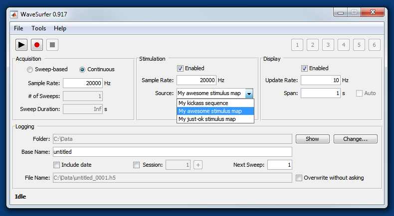
Stimulation (i.e. the production of output signals) can be turned on by checking the “Enabled” checkbox in the Stimulation panel of the main WaveSurfer window, shown below. The “Source:” field allows the user to select the stimulus map to be used in the upcoming run. A stimulus map defines the output signals that will go out each output terminal. (The user can also select a stimulus sequence as the output source. A stimulus sequence is a sequence of stimulus maps, to be used one after the other.) Clicking the “Edit…” button will launch the Stimulus Library window, which allows the user to define one or more stimulus maps. (The Stimulus Library can also be launched from Tools > Stimulus Library… in the main window.)

Stimulus Library
The stimulus library allows one to flexibly define what signals will go out what outputs. It traffics in three kinds of entity: stimuli, maps, and sequences.
Stimuli
A stimulus is a single time-varying signal which can be used as an output, such as a sine wave or a square wave. The figure below shows the stimulus library window when a single stimulus is selected. In WaveSurfer, each stimulus has a name that uniquely identifies it (“My Awesome Pulse” in the figure below). It also has a functional form (“Square Pulse”, “Ramp”, “Sine”, etc.), a delay, a duration, an amplitude, and a DC offset. The delay determines how long WaveSurfer will wait before starting the stimulus. The duration determines how long the stimulus will last. The amplitude determines how large the stimulus will be. The DC offset is a constant that is added to the stimulus. (But note that the DC offset is only added in the window of time between t=delay and t=delay+duration. The stimulus is always zero outside this window, regardless of the settings of the other parameters.)
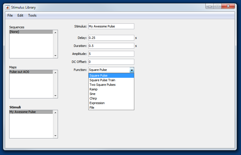
Some functional forms have additional parameters. For instance, the sine stimulus has a frequency parameter; the chirp stimulus has an initial frequency and and final frequency.
Note that the parameters of a stimulus do not have to be simple
numbers: They can also be Matlab expressions that contain the sweep
index (represented by the variable i), which is one on
the first sweep, two on the second sweep, etc. For instance, 2*i
and 10*(i-6) are both legal values for any parameter. So
are things like mod(i,2), which is one on odd-numbered
sweeps and zero on even-numbered sweeps. These can be used to easily
produce ‘ladder’ stimuli such as those used in voltage-clamp
experiments. For instance, in a run with 11 sweeps, a square pulse of
amplitude 10*(i-6) used as a voltage command would
hyperpolarize the cell -50 mV below holding potential on sweep 1, -40
mV on sweep 2, etc., and finally +50 mV on sweep 11.
Two functional forms deserve special attention: “Expression” and
“File”. The expression form allows one to specify the output as a
Matlab expression in the variables t, the time since the
start of the sweep in seconds, and i, the sweep index.
For instance, if you wanted a sine wave superimposed on a slower sine
wave, this can be achieved with the expression 5*sin(2*pi*0.1*t)+sin(2*pi*2*t),
as shown below. (You can see a preview of any stimulus in WaveSurfer
by going to Tools > Preview… in the Stimulus Library window.)

More exotically, if you wanted a Bessel-function stimulus (although
I’m not sure why you would…), this can be achieved with the expression
besselj(1,5*t), as shown below. (You can see a preview of
any stimulus in WaveSurfer by going to Tools > Preview… in the
Stimulus Library window.) In addition to calling built-in functions,
you can also call any user-defined functions on the Matlab path.

The “File” functional form allows you to read a signal from a .wav
file and output it from WaveSurfer. An example is shown below, using a
.wav file containing a recording of Godzilla’s
trademark bellow from one of those classic movies. (This file
can be found at +ws\+test\+hw\godzilla.wav in the
WaveSurfer directory.) A .wav file specifies the sampling rate of the
audio it contains, and this signal is linearly resampled onto the
WaveSurfer stimulation sampling rate before being output. Further, the
data is interpreted as ranging from -1 to +1. The data in the .wav
file is treated as defining a ‘core’ stimulus that is non-zero in a
window from t=0 to t=(number of samples in file)*(sampling rate in
file). This core stimulus is then multiplied by the specified
amplitude parameter, is offset by the given DC offset, is set to zero
for times greater than the specified duration, and the resulting
function is then delayed by the given delay parameter. (This is
actually how all stimuli are generated in WaveSurfer. A core function
is defined for all possible values of (continuous) time, and this
function is then scaled, offset, windowed, and delayed by the given
amounts, and is then sampled at the needed time points.)

Stimulus Maps
A stimulus map associates output channels with stimuli. For instance, the map below is named “My awesome stimulus map” and outputs the stimulus “Sine plus sine = fun” from AO0, and “Godzilla!” from AO1. (You can also use Tools > Preview… to preview a stimulus map.)

Note that a stimulus map has its own duration (to the right of the map name in the above figure), which is independent of the duration and delay of the stimuli that are included in the map. In sweep-based mode, the durations of all maps are fixed to the sweep duration. In continuous mode, the map duration is an independent parameter, which can be set to anything the user likes. If a stimulus in the map has an “end time” (the stimulus delay+duration) before the end of the stimulus map, then that channel is padded with zeros until the end of the map. If a stimulus in the map has an end time after the end of the map, the stimulus is truncated. That is, the duration of the map ‘overrules’ the end time of any of the stimuli in the map.
You may have noticed that each indivdual stimulus does not have units associated with it. This is because the units of a stimulus are determined by the channel it is associated with in the map. (Recall that each analog output channel has units associated with, set via Tools > Device & Channels… in the main menu.) If the units of the channel are mV, then those are the units of the stimulus, at least in the context of that map. But note that the same stimulus can be used in multiple maps, and can be associated with a different output channel in each. So the same stimulus can have different units in different maps. Therefore, it does not make sense to associate units with individual stimuli in isolation.
A stimulus map also provides the ability to scale each stimulus, independently of the stimulus amplitude. This facility is provided by the “Multiplier” column in the stimulus map.
In the Stimulus Library, the Edit menu provides options to add and delete maps, and to add and delete channels from maps.
You can assign any stimulus to any channel, whether the channel is analog or digital. For digital channels, the stimulus is thresholded at a value of 0.5. Any sample points greater than or equal to 0.5 are output as TTL true (5 V), any sample points less than 0.5 are output as TTL false (0 V). Crude, but effective.
Stimulus Sequences
Stimulus sequences enable the user to output different stimulus maps on different sweeps of a run, one after the other. An example of a stimulus sequence containing two stimulus maps is shown below.

In the Stimulus Library, the Edit menu provides options to add and delete sequences, and to add and delete maps from a sequence.
Stimulation Source
Once all your desired stimuli are in the stimulus library, you select which sequence or map will be output using the “Source” pop-up menu in the Stimulation panel of the main WaveSurfer window, as shown below. Note that either a sequence or a map can be the stimulation source, but not an individual stimulus. The “Repeats” checkbox determines whether the sequence/map will be used repeatedly or only once. For instance, if the stimulation source is a sequence with 2 maps in it, the Repeats checkbox is unchecked, and you perform a sweep-based run with 10 sweeps in it, there will be output only on the first two sweeps—the last eight sweeps will have no output. In contrast, if the Repeats checkbox is checked, the sequence will be repeated five times, and there will be output on all the sweeps. The Repeats checkbox is checked by default.
Saving a Protocol
All of the settings we’ve talked about so far are all part of a WaveSurfer “protocol”—the collection of settings that collectively describe a certain kind of experiment or experimental trial. Essentially all of the current WaveSurfer settings can be saved to a “protocol file” via the File > Save Protocol menu item (shown in the figure below). The only exceptions to this rule are the settings in the Logging panel, and the configuration of the Fast Protocol buttons (the buttons numbered 1–6 in the upper right of the main window). The logging settings are not saved to the protocol file because they are likely to change from day to day, even though the same type of experiment is being conducted. The Fast Protocol buttons (whose function will be described in more detail below) are used to quickly load protocol files, and so it makes little sense to store their settings in a protocol file itself. In addition to the settings, the position and visibility of all windows are also saved to the protocol file.

After being saved to a protocol file (which for historical reasons have the extension .cfg), a protocol can be re-loaded using the File > Open Protocol… menu item (shown in the figure above).
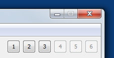
Fast Protocols
When you are doing experiments with WaveSurfer, you will probably have a handful of protocols that you want to use in the course of a single experiment. To allow you to quickly switch between protocols, WaveSurfer has a feature called “Fast Protocols”. Once set up, fast protocols allow you to load a protocol file simply by clicking on one of the buttons numbered 1–6 in the upper right corner of the main WaveSurfer window (shown below, with the first three buttons enabled).
To set up a fast protocol, select Tools > Fast Protocols… in the main WaveSurfer window. You should see the Fast Protocols window appear, as shown below.

Click the “Select File…” button, and select an existing protocol file. After this, the fast protocol button labelled “1” in the main window will be ungrayed, and clicking this button will load the selected protocol file. Additionally, the “Action” column in the Fast Protocols window allows you to select an action to be performed after loading the protocol file. This can be “Do Nothing” (the default), “Play”, or “Record”. Selecting “Play” or “Record” will cause a run to start immediately after pressing the fast protocol is loaded. This is equivalent to automatically pressing the play or record button right after loading the protocol file.
User Settings
Many applications have ‘preferences’ that are settable by the user. These are typically stored on a per-user basis, so that each user can have their own preferences. WaveSurfer has something like this, only slightly more awkward. The user can save a ‘user settings’ file which contains their preferences (File > Save User Settings), and load these again as needed (File > Open User Settings…). At present, the only thing stored in the user settings file is the fast protocol settings, i.e. the protocol file associated with each button, and the post-load action (“Do Nothing”, “Play”, or “Record”).
Triggers
WaveSurfer provides a good deal of flexibility in how sweeps are triggered. They can be triggered automatically (the default), based on a precise internal timer, or in response to an external TTL signal. The triggering options can be changed by selecting Tools > Triggers… in the main WaveSurfer window. This launches the window shown below.

There is a configurable trigger for acquisition, and one for stimulation. The trigger determines whether triggering for that entity will use WaveSurfer’s built-in trigger, be generated by an onboard counter timer, or be externally supplied, and what the triggering parameters are in either case. WaveSurfer’s built-in trigger fires as soon as WaveSurfer is ready to perform a sweep. It is the default trigger, and has no parameters. For a ‘counter’ trigger (an internally-generated, precisely-timed, repetitive trigger), parameters include the time between trigger edges, the number of trigger edges to be generated, and the NI counter number that actually generates the trigger signal. For an external trigger, the parameters include the PFI line the external trigger will be coming in on, and whether rising or falling edges will be used as the triggers.
The built-in trigger is output from the DAQ board on PFI8. If needed, this can be used to trigger external devices that should be synchronized with WaveSurfer. “PFI” stands for “programmable function interface”. WaveSurfer uses these lines for triggering, and only for triggering. On many NI boards, the PFI terminals are multiplexed with the P1 and P2 digital I/O lines. WaveSurfer always uses these lines as PFI lines (i.e. for triggering), never as general-purpose digital lines.
If we add a counter trigger (using the “Add” button under the “Counter Triggers” table) and an external trigger (using the “Add” button under the “External Triggers” table), the Triggers window looks like the figure below.

In the figure above, one can see the newly-added counter trigger in the upper right, along with its associated NI device name, NI counter number, number of repeats to generate, interval between repeats, PFI line (for outputting the trigger), and edge polarity (rising or falling). One can also see the newly-added external triggers in the lower right, along with its associated NI device, PFI line, and edge polarity.
Up to this point in the manual, we’ve referred to “sweeps” when speaking both of acquisition and stimulation. For sweep-based acquisition, this is fitting and proper, since acquisition sweeps and stimulation “sweeps” are always of the same duration, and are always triggered simultaneously. But going forward, it will be useful to distinguish between acquisition sweeps and stimulation “episodes”. A stimulation episode is completely analogous to an acquisition sweep, but for in continuous acquisition mode the two are not of the same duration, nor are they (necessarily) triggered at the same time.
To select the trigger used for acquisition, the user selects it from the “Scheme:” drop-down menu in the Acquisition section of the Triggers window (upper left; see figure below). Note that only the built-in trigger and the external triggers (not counter triggers) can be used as the acquisition trigger. This was a conscious design choice. If you need to perform stimulation episodes with precise inter-episode intervals, you should change the acquisition mode to continuous (in the main window), then use a counter trigger to trigger each stimulation episode. This will yield one long sweep with all the stimulation episodes within it. (One advantage of this is that you collect data between the stimulation episodes, so that if anything unexpected happens during this time, you will have a record of it.) When using the built-in trigger combined with sweep-based acquisition, note that there will be a somewhat variable interval between sweeps, while WaveSurfer prepares for the next sweep. If this variability is a problem, we recommend switching to continuous acquisition with stimulation episodes triggered by a counter trigger.

In sweep-based acquisition, the stimulation trigger is identical to the acquisition trigger. If continuous acquisition is selected in the main window, the Stimulation > “Use acquisition scheme” checkbox in the Triggers window ungrays, and the user may uncheck it if desired. Doing so allows the stimulation trigger to be different from the acquisition trigger. To select the trigger used for stimulation, the user selects it from the “Scheme:” popup menu. For instance, the user could use the built-in trigger for acquisition, and an external trigger for stimulation.

When external triggering is used, any acquisition triggers that arrive during an ongoing acquisition sweep are ignored. Similarly for stimulation triggers and episodes.
When the stimulation trigger is a counter trigger, the counter is started at the start of the acquisition sweep, regardless of how the acquisition sweep is triggered. Note that it is only possible to have the stimulation trigger be a counter trigger if using continuous acquisition. (Because the stimulation trigger is forced to be the same as the acquisition trigger in sweep-based mode, and the acquisition trigger cannot be a counter trigger.) Thus when the acquisition trigger is external, and the stimulation trigger is a counter trigger, the counter is started at the start of the acquisition sweep. I.e. it is not started until the external trigger starts the (single) acquisition sweep.
If both the acquisition and the stimulation triggers are external, but they are different, note that it is possible for stimulation to occur when data is not being acquired. If this is undesirable, you need to somehow ensure that the stimulation triggers only occur when a sweep has been triggered and is not yet over. Alternatively, you could simply use continuous acquisition.
Electrodes
Thus far, all of the WaveSurfer capabilities we’ve talked about are useful for general data acquisition, whether that data represents the membrane potentials of neurons, audio data from a microphone array, or whatever. We will now discuss some WaveSurfer features that are specific to neurophysiology data acquisition.
In neurophysiology experiments, a set of inputs and outputs are often associated with a single electrode. For instance, some patch-clamp amplifiers have four separate BNC terminals for a single electrode: one output for measured membrane potential, one output for the injected current, one input for the command current, and one input for the voltage clamp command. Other amplifiers multiplex these signals, using one output BNC and one input BNC. The output BNC reflects the membrane potential in current clamp mode and the injected current in voltage clamp mode, the input BNC provides the current command in current clamp mode and the voltage command in voltage clamp mode. But in all these cases, several signals pertain to one electrode.
WaveSurfer can handle all the signals associated with a single electrode in a coordinated manner if it ‘knows’ which signals go to the same electrode. This information can be specified in the “Electrodes” window, available under Tools > Electrodes… in the main WaveSurfer window. On first launch, the Electrodes window looks as shown below.

A single electrode can be added by clicking the “Add” button in the lower left.
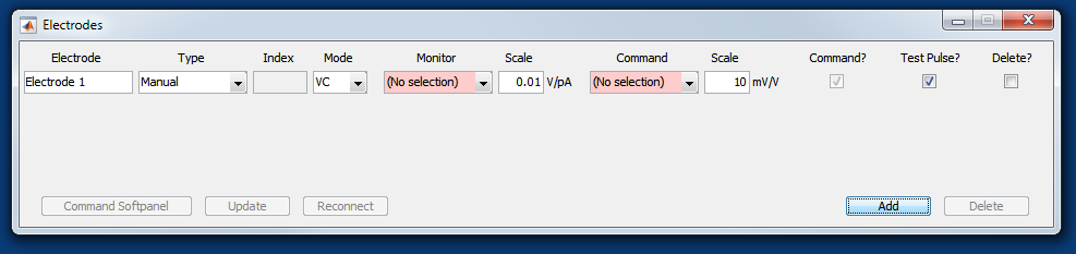
A newly-created electrode is assumed to be a “Manual” electrode (as opposed to a computer-controlled one), and is assumed to be in voltage clamp (VC) mode. You’ll note that no channel has been selected to be the current monitor channel when in VC mode, nor has any channel been selected to be the voltage command channel when in VC mode. (The reddish background indicates that this is problematic in some way.) If we select AI0 to be the VC monitor channel, and AO0 to be the VC command channel, the figure looks as shown below.

With the electrode configured this way, the Device & Channels window looks as shown below. Note that the units of channel AI0 and AO0 are set to pA and mV, respectively, as is appropriate for a current monitor and a voltage command. Further, the Units edit box is grayed to indicate its value has been overridden by the value in the Electrodes window. Also, the scales of both channels are set to the values specified in the Electrodes window, and these fields are also grayed. This is generally the case: if a channel is claimed by an electrode, its units and scale are controlled by the electrode settings, and any pre-existing settings are overridden. (The old settings are still remembered, however, and will be restored if the channel is subsequently ‘released’, for instance if you delete the electrode.)

To set the electrode channels for current clamp (CC) mode, you have to switch the electrode mode to CC in WaveSurfer. The monitor channel for CC mode does not have to be the same as for VC mode, but it can be. (Which way you configure this will depend on how your amplifier works.) Similarly, the command channel for CC mode does not have to be the same as for VC mode, but it can be. If an AI channel is the monitor channel for both VC and CC mode, its units and scale factor will be switched when you switch from VC to CC mode and back. Similarly for an AO channel that is the command channel for both VC and CC mode. In the figure below, we’ve configured the electrode CC channels to be the same as the VC channels, but note that the scale factor and units are different when the electrode is set to CC mode. (OK, one of the scale factors is the same, but that’s mere happenstance.)

Test Pulse
One WaveSurfer feature that becomes useful only after you have associated specific channels with electrodes is the “Test Pulse” window, launched via Tools > Test Pulse… in the main WaveSurfer window. This allows you to deliver a repetitive test pulse stimulus using the configured electrode, which is useful when patching onto a cell. The figure below shows a typical test pulse response in voltage clamp mode, with the electrode in the bath. (We actually used a model cell in “bath” mode to make these screenshots, but real data should looks grossly similar.)
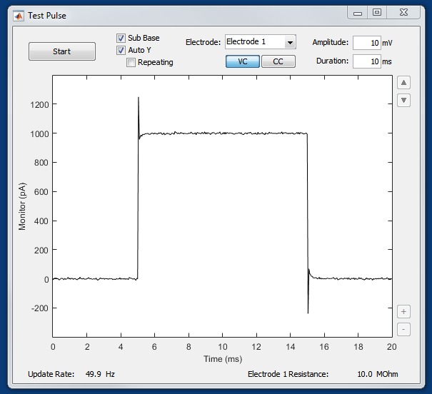
The “Duration:” field sets the duration of the test pulse. The duration of the complete output waveform is always twice this duration, with the pulse itself centered in time. The “Sub Base” checkbox controls whether or not the baseline level is subtracted off of the monitor signal before displaying it. The baseline level is the average monitor signal during the first half of the pre-pulse interval. E.g. if the pulse duration is 10 ms, the pre-pulse interval will be 5 ms long, and the baseline will be calculated from the first 2.5 ms of the monitor signal. When “Sub Base” is checked, the baseline is computed and subtracted out on each sweep.
The “Auto Y” checkbox, when checked, causes WS to set the y axis limits based on the range of the acquired monitor signal. When unchecked, the y axis limits do not change depending on the monitor signal. (When “Auto Y” is unchecked, the buttons of the right side of the plot ungray, and can be used to zoom in and out, and to shift the y axis limits up and down.) The “Auto Y” checkbox is checked by default.
The “Repeating” checkbox (under the “Auto Y” checkbox), which is only ungrayed if “Auto Y” is checked, determines whether the y axis limits are adjusted after every sweep, or only after the first sweep. If “Repeating” is unchecked (the default), the y-axis limits are set after the first sweep, and left unchanged afterward. If “Repeating” is checked, the y axis limits are updated continually while the test pulse is running.
The resistance faced by each electrode is displayed under the test pulse plot. In VC mode, resistance is determined by first calculating the mean current delivered during the baseline interval (the first half of the pre-pulse interval record), then calculating the mean current delivered during the “pulse” interval, the last fourth of the test pulse. (These two intervals have the same duration.) The baseline current is subtracted from the pulse current to calculate the current step amplitude, and the resistance is equal to the voltage command step amplitude (set in the “Amplitude:” edit box) divided by the current step amplitude. The calculation of resistance is similar in CC mode, except the (measured) voltage step amplitude is divided by the (prespecified) current command step amplitude.
By default, the test pulse is delivered to all electrodes simultaneously, and the resistance of each electrode is displayed at the bottom of the test pulse window. Only one electrode at a time has its monitor waveform displayed, however: the one specified by the “Electrode:” popup menu in the Test Pulse window. Each electrode ‘remembers’ its own test pulse amplitude, and these be set by selecting each electrode in turn. using the popup menu. If you would like to apply the test pulse only to a subset of electrodes, the “Test Pulse?” checkbox in the Electrodes window can be unchecked for the electrode(s) you do not wish to deliver the test pulse to.
The electrode mode (VC or CC) can also be changed in the Test Pulse window. This mode is kept in sync with the mode as displayed in the “Electrodes” window.
Computer-controlled electrodes
Some microelectrode amplifiers can be controlled only via buttons, switches, and dials on the amplifier itself. We call these ‘manual’ amplifiers. For this type of amplifier, the user must take care that each electrode’s mode in WS is the same as that electrode’s true mode, as set in the amplifier. Otherwise, test pulses and other stimuli will have strange (and perhaps dangerously large) amplitudes, and monitored signals will generally have the wrong scaling and units.
Other microelectrode amplifiers can be controlled via an attached computer, and for some of these WaveSurfer can communicate with the amplifier directly to keep the WaveSurfer electrode mode in sync with the true electrode mode (as set in the amplifier). Furthermore, for supported amplifiers WaveSurfer can automatically read scaling factors directly from the amplifier, and in some cases set them also.
Two types of amplifiers are currently supported in WaveSurfer: Axon MultiClamp amplifiers and Heka EPC 10 amplifiers. For Axon MultiClamp amplifiers, WaveSurfer communicates with the MultiClamp Commander ‘softpanel’ software that is normally used to control the amplifier. To inform WaveSurfer that an electrode is an Axon MultiClamp electrode, you select “Axon Multiclamp” [sic] from the “Type” popup menu for that electrode (in the Electrode window).
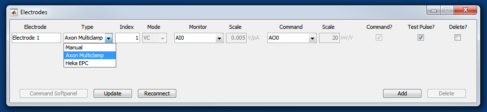
When you do this, you will note that the “Mode” and “Scale” controls are grayed, and the “Update” and “Reconnect” buttons are enabled. This is because WaveSurfer’s current Axon MultiClamp support only allows it to read parameters from the amplifier, not to write them. So the mode and scales are now read from the amplifier, and to set them the user must use the MultiClamp Commander softpanel. After changing parameters with the softpanel, the user must press the “Update” button to prompt WaveSurfer to re-read the mode and scales from the amplifier. If MultiClamp Commander is shutdown, or the amplifier itself is power cycled, it may be necessary to press the “Reconnect” button to re-establish communication with the amplifier.
For a Heka EPC amplifier, WaveSurfer communicates with Heka’s softpanel software, EpcMaster. (WaveSurfer can also communicate with Heka PatchMaster, a data-acquisition-plus-softpanel application.) The user should set the “Type” popup menu to “Heka EPC” (shown below).

The “Mode” and “Scale” controls are grayed, and the “Command Softpanel”, “Update”, and “Reconnect” buttons are enabled. The “Command Softpanel” button is a togglebutton, and by default it is off. In this mode, the mode and scales are read from the amplifier, and to set them the user must use the Heka softpanel software. After changing parameters with the softpanel, the user must press the “Update” button to prompt WaveSurfer to re-read the mode and scales from the amplifier. If the Heka softpanel software is shutdown, or the amplifier itself is power cycled, it may be necessary to press the “Reconnect” button to re-establish communication with the amplifier.
If the user presses the “Command Softpanel” togglebutton, it will switch to the on state (shown below; note the blue accent on the “Command Softpanel” button).

In this mode (‘command mode’), the electrode mode popup menu is enabled, as are the scale edit boxes. In command mode, WaveSurfer can command the Heka softpanel to change the electrode mode and the scale factors. The Heka softpanel user interface is disabled in this mode.
User Code
One of the primary selling points of WaveSurfer is its ability to call custom user code at various points during data acquisition. This enables you to easily perform online data analysis and also perform closed-loop experiments. In order to call your own code, you must create something called a ‘user class’.
At this point, a bit of background on object-oriented programming may be helpful. Predictably, object-oriented programming involves the creation of software ‘objects’. These are a lot like structs in Matlab, in that they contain a number of named fields, each of which holds some data. (These fields are called ‘properties’ when they’re part of an object, for reasons that are complicated.) But each object also has functions associated with it, which are called ‘methods’. The idea is that you write a method for each thing you might like to do with the object, so the object is a self-contained little ball of data combined with the code used to manipulate that data. You often want to create several objects that all the share the same properties and methods, so to create an object, you must first create a ‘class’, which specifies what properties and methods each object will have. Once you’ve defined a class, you can use it to create as many objects as you want. All the objects derived from the same class will have the same fields and methods, but the values stored in the fields can differ from object to object. Each object is called an ‘instance’ of its class, and we say that we ‘instantiate’ an object from the class.
An example WaveSurfer user class definition can be found in the WaveSurfer installation directory under:
+ws/+examples/ExampleUserClass.m
The complete text of this class is shown below.
classdef ExampleUserClass < ws.UserClass

    % This is a very simple user class.  It writes to the console when
    % things like a sweep start/end happen.

    % Information that you want to stick around between calls to the
    % functions below, and want to be settable/gettable from outside the
    % object.
    properties
        Greeting = 'Hello, there!'
    end  % properties

    % Information that you want to stick around between calls to the
    % functions below, but that only the methods themselves need access to.
    % (The underscore in the name is to help remind you that it's
    % protected.)
    properties (Access=protected)
        TimeAtStartOfLastRunAsString_ = ''
    end

    methods
        function self = ExampleUserClass(rootModel)
            % creates the "user object"
            fprintf('%s  Instantiating an instance of ExampleUserClass.\n', ...
                    self.Greeting);
        end

        function delete(self)
            % Called when there are no more references to the object, just
            % prior to its memory being freed.
            fprintf('%s  An instance of ExampleUserClass is being deleted.\n', ...
                    self.Greeting);
        end

        % These methods are called in the frontend process
        function startingRun(self,wsModel,eventName)
            % Called just before each set of sweeps (a.k.a. each
            % "run")
            self.TimeAtStartOfLastRunAsString_ = datestr( datetime() ) ;
            fprintf('%s  About to start a run.  Current time: %s\n', ...
                    self.Greeting,self.TimeAtStartOfLastRunAsString_);
        end

        function completingRun(self,wsModel,eventName)
            % Called just after each set of sweeps (a.k.a. each
            % "run")
            fprintf('%s  Completed a run.  Time at start of run: %s\n', ...
                    self.Greeting,self.TimeAtStartOfLastRunAsString_);
        end

        function stoppingRun(self,wsModel,eventName)
            % Called if a sweep goes wrong
            fprintf('%s  User stopped a run.  Time at start of run: %s\n', ...
                    self.Greeting,self.TimeAtStartOfLastRunAsString_);
        end

        function abortingRun(self,wsModel,eventName)
            % Called if a run goes wrong, after the call to
            % abortingSweep()
            fprintf('%s  Oh noes!  A run aborted.  Time at start of run: %s\n', ...
                    self.Greeting,self.TimeAtStartOfLastRunAsString_);
        end

        function startingSweep(self,wsModel,eventName)
            % Called just before each sweep
            fprintf('%s  About to start a sweep.  Time at start of run: %s\n', ...
                    self.Greeting,self.TimeAtStartOfLastRunAsString_);
        end

        function completingSweep(self,wsModel,eventName)
            % Called after each sweep completes
            fprintf('%s  Completed a sweep.  Time at start of run: %s\n', ...
                    self.Greeting,self.TimeAtStartOfLastRunAsString_);
        end

        function stoppingSweep(self,wsModel,eventName)
            % Called if a sweep goes wrong
            fprintf('%s  User stopped a sweep.  Time at start of run: %s\n', ...
                    self.Greeting,self.TimeAtStartOfRunAsString_);
        end

        function abortingSweep(self,wsModel,eventName)
            % Called if a sweep goes wrong
            fprintf('%s  Oh noes!  A sweep aborted.  Time at start of run: %s\n', ...
                    self.Greeting,self.TimeAtStartOfLastRunAsString_);
        end

        function dataAvailable(self,wsModel,eventName)
            % Called each time a "chunk" of data (typically 100 ms worth)
            % has been accumulated from the looper.
            analogData = wsModel.Acquisition.getLatestAnalogData();
            digitalData = wsModel.Acquisition.getLatestRawDigitalData();
            nScans = size(analogData,1);
            fprintf('%s  Just read %d scans of data.\n',self.Greeting,nScans);
        end

        % These methods are called in the looper process
        function samplesAcquired(self,looper,eventName,analogData,digitalData)
            % Called each time a "chunk" of data (typically a few ms worth)
            % is read from the DAQ board.
            nScans = size(analogData,1);
            fprintf('%s  Just acquired %d scans of data.\n',self.Greeting,nScans);
        end

        % These methods are called in the refiller process
        function startingEpisode(self,refiller,eventName)
            % Called just before each episode
            fprintf('%s  About to start an episode.\n',self.Greeting);
        end

        function completingEpisode(self,refiller,eventName)
            % Called after each episode completes
            fprintf('%s  Completed an episode.\n',self.Greeting);
        end

        function stoppingEpisode(self,refiller,eventName)
            % Called if a episode goes wrong
            fprintf('%s  User stopped an episode.\n',self.Greeting);
        end

        function abortingEpisode(self,refiller,eventName)
            % Called if a episode goes wrong
            fprintf('%s  Oh noes!  An episode aborted.\n',self.Greeting);
        end
    end  % methods

end  % classdef
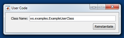
To create a user object of class ExampleUserClass, go
to Tools > User Code… in the main WaveSurfer window. The “User
Code” window will appear (shown below). Type
“ws.examples.ExampleUserClass” into the “Class Name:” edit box and hit
the “Enter” key. This creates an object of class ExampleUserClass, and
registers it as the WaveSurfer user object. The string “Hello there!
Instantiating an instance of ExampleUserClass.” will be printed to the
Matlab console.
(Why do you have to type “ws.examples.ExampleUserClass” instead of “+ws/+examples/ExampleUserClass.m”? Because a directory that starts with “+” is treated as a ‘package’ by Matlab, and Matlab uses the “.” syntax to refer to functions and classes within packages. In this case, “examples” is a subpackage within the “ws” package.)
In the methods section of the above code, you will
find a bunch of Matlab functions. Each of these is a method, and once
the user object is registered with WaveSurfer, WaveSurfer will call
methods with particular names at particular times. For instance, the
method startingRun() is called at the start of each run,
as the name implies. The table below lists nine of the user methods,
and when they are called.
| Method | When called |
|---|---|
startingRun() |
Called at the start of each run |
completingRun() |
Called at the end of a run if the run completed normally |
stoppingRun() |
Called at the end of a run if the run was stopped by the user |
abortingRun() |
Called at the end of a run if the run is stopping because something went wrong |
startingSweep() |
Called at the start of each sweep |
completingSweep() |
Called at the end of a sweep if the sweep completed normally |
stoppingSweep() |
Called at the end of a sweep if the sweep was stopped by the user |
abortingSweep() |
Called at the end of a sweep if the sweep is stopping because something went wrong |
dataAvailable() |
Called each time a ‘chunk’ of data (usually about 100 ms worth) has been acquired. |
The methods in ExampleUserClass mostly just call fprintf()
to notify the user that they have been called. The dataAvailable()
method also gets the just-acquired data and prints out how many new
samples are available. You should perform a few runs with the ExampleUserClass
user object and examine the Matlab console to convince yourself that
WaveSurfer is indeed calling the various methods at the appropriate
times.
Note that all the methods in the table above take a wsModel
argument. When these methods are called, wsModel is a reference to the
WaveSurfer model object, an instance of class ws.WavesurferModel
[sic]. This allows the user object methods to access information about
the current WaveSurfer settings and state.
What about properties? Properties provide a way for user object
methods to exchange information. For instance, you might want to
perform some expensive computation in startingRun(),
store the result in a property, and then read from this property in
each call to completingSweep(). This would enable you to
compute the value only once per run, rather than once per sweep. In
this way, properties are a bit like global variables, but they do a
better job of keeping out of the way of code that doesn’t access them.
The property TimeAtStartOfLastRunAsString_ in ExampleUserClass
is an example of this sort of property. In the startingRun()
method, we get the current time using the built-in datetime()
function, then store it (as a string) in the property TimeAtStartOfLastRunAsString_.
Many of the other methods in the class then read TimeAtStartOfLastRunAsString_
and print its value. (Granted, calling datetime() is not
a particularly expensive computation, but the example shows how to use
properties to share the results of a computation in one method with
other methods.)
When TimeAtStartOfLastRunAsString_ is declared (near
the top of ExampleUserClass.m), the properties
block it is declared in is marked as (Access=protected).
This makes it so that only methods of class ExampleUserClass
can access the property. (Geeks: Yeah, I know that’s not exactly
true, but it’s close enough for the present purposes.) This protects
it from being modified in ways that the class author may not have
anticipated. As a convention, I like to add an underscore to the names
of such properties, but this is just a convention—it is not required.
Another use of properties is to hold parameters that the user might
want to change. In ExampleUserClass, the property Greeting
is like this. It is set to the value 'Hello, there!'
when the object is created, but the user can then change it. Once
changed, the new value will be used on subsequent calls to the object
methods, changing the text that is printed. The properties
block that Greeting is declared in is not marked with
any qualifiers like (Access=protected), which means that
Greeting is a ‘public’ property: It can be read and
written by code outside the object, and can also be modified directly
from the Matlab command line.
How would the user change the value of Greeting?
Currently, it’s a bit of a pain. The users selects File > Export
Model and Controller to Workspace from the main menu. This introduces
the variables wsModel and wsController
into the main Matlab workspace. Then, at the Matlab command line, the
command
 wsModel.UserCodeManager.TheObject.Greeting =
            'Hola!' ;
would change the Greeting to 'Hola!',
which would then be printed on subsequent calls to ExampleUserClass
methods. (Note that after you do File > Export Model and Controller
to Workspace, you will have to do
clear wsModel wsController ;
after you quit WaveSurfer in order to fully clear WaveSurfer from memory, and to close the WaveSurfer satellite windows.) It is also possible to write a custom GUI (that is launched when your user object is created) that allows the user to change parameter values using a GUI, but describing how to do this is beyond the scope of this manual.
What about the other functions in the methods section
of ExampleUserClass? The very first one is named ExampleUserClass,
and is the constructor. It is called when the the user object
is first created. (The string “Instantiating an instance of
ExampleUserClass.” was printed to the Matlab console when you created
the ExampleUserClass object because of the call to fprintf()
in the ExampleUserClass constructor.)
It is somewhat more involved to explain the rest of the methods in ExampleUserClass.
First, some background: WaveSurfer consists of three processes: the
frontend, the looper, and the refiller. The frontend is the one you
interact with directly and also handles logging data to disk, the
looper does the essential data acquisition and handles the on-demand
outputs, and the refiller makes sure the output buffers for the timed
outputs get filled as needed. The frontend contains a single instance
of class ws.WavesurferModel, the looper process contains a single
instance of ws.Looper, and the refiller process contains a single
instance of ws.Refiller.
When you create a user object, it is initially created only in the
frontend. But when you start a run, that causes a user object to be
created in the looper, and one to be created in the refiller. All
these objects are instances of the same class, so they all have the
same methods. But here’s the critical part: almost all of the methods
are called by only the frontend, or only the looper, or only the
refiller. In particular, all the methods listed in the table above are
only called in the frontend. (But note that the constructor and
the delete() method can be called in any of the three
processes.)
There is only one method that is called only by the looper: samplesAcquired().
It is called very frequently, typically every few milliseconds. It is
intended to be used to implement feedback loops, which generally
require minimal latency. Whereas the frontend methods have an argument
called wsModel which contains a reference to the
frontend model object (of class ws.WavesurferModel), the
samplesAcquired method has an argument called looper,
which contains a reference to the looper model object (of class ws.Looper).
The looper model object is similar to the frontend model object, but
only contains subsystems that are relevant to the looper. So, for
instance, the looper model object contains no Logging
property, because logging data to disk is handled by the frontend.
The methods called only in the refiller are listed in the table
below, along with when each is called. They are analogous to the
frontend methods called at the start/end of an acquisition sweep.
Recall that a stimulation episode is analogous to an acquisition
sweep, and in some situations they are essentially identical. These
methods each have an argument called refiller, which
contains a reference to the refiller model object (of class ws.Refiller).
The refiller model object is similar to the frontend model object or
the looper model object, but only contains subsystems that are
relevant to the refiller. So, for instance, the refiller model object
contains no Acquisition property, because data
acquisition is handled by the frontend and the looper.
| Method | When called |
|---|---|
startingEpisode() |
Called at the start of each episode |
completingEpisode() |
Called at the end of an episode if the episode completed normally |
stoppingEpisode() |
Called at the end of an episode if the episode was stopped by the user |
abortingEpisode() |
Called at the end of an episode if the episode is stopping because something went wrong |
Creating your own user class
To create your own user class, we recommend copying +ws/+examples/ExampleUserClass.m
to some convenient location on the Matlab path, renaming it, and then
customizing it to suit. You will then have to change the class
name in the “User Code” window. After that, WaveSurfer should
create an instance of your user class, and call its methods during a
run.
Useful WavesurferModel Properties and Methods
As mentioned before, the wsModel argument that is
handed to the frontend methods is an instance of the ws.WavesurferModel
class. This object represents (almost) the entire current state of the
WaveSurfer application. We won’t describe all of this state, but below
are some properties and methods that are particularly useful. Note
that all the same properties and methods are also available from the
command line if the user has exported the model and controller to the
Matlab workspace.
wsModel.Acquisition.SampleRate
This is the acquisition sampling rate in Hz. User can both get this value and also set it, although generally it should not be set in the midst of a run.
wsModel.Acquisition.SweepDuration
The sweep duration, in seconds. User can both get this value and
also set it, although generally it should not be set in the midst of a
run. If set to inf, acquisition mode is set to
continuous.
wsModel.Acquisition.NAnalogChannels
The number of analog input channels, whether active or not. A double scalar.
wsModel.Acquisition.NDigitalChannels
The number of digital input channels, whether active or not. A double scalar.
wsModel.Acquisition.AnalogChannelNames
The name of each analog input channel, whether active or not, in the
order of channel creation. A cell array of strings, of size 1 x
NAnalogChannels.
wsModel.Acquisition.DigitalChannelNames
The name of each digital input channel, whether active or not, in
the order of channel creation. A cell array of strings, of size 1
x NDigitalChannels.
wsModel.Acquisition.IsAnalogChannelActive
A logical row array indicating whether each analog input channel is
active or not. Of size 1 x NAnalogChannels.
wsModel.Acquisition.IsDigitalChannelActive
A logical row array indicating whether each digital input channel is
active or not. Of size 1 x NDigitalChannels.
wsModel.Acquisition.AnalogChannelUnits
The native units of each analog input channel, as a string. A cell
array of size 1 x NAnalogChannels.
wsModel.Acquisition.AnalogChannelScales
The scale factor for converting each analog input from volts to
native units. Each element is in units of volts per AnalogChannelUnits
(above). A double array of size 1 x NAnalogChannels.
wsModel.Acquisition.getLatestAnalogData()
This returns the most recent chunk of analog data, as seen by the
frontend. The looper acquires data in as-small-as-possible chunks, and
then sends the data to the frontend when it has accumulated a number
of these chunks. Typically a frontend chunk is about 100 ms long.
This data is nScans x nChannels, where nScans
is the number if time points, and is a double array. The data has
already been scaled, and is in the units specified in the Device &
Channels window.
wsModel.Acquisition.getLatestRawAnalogData()
This returns the most recent chunk of analog data, as seen by the
frontend (see above). This data is nScans x nChannels,
where nScans is the number if time points, and is an
int16 array. Each sample represents the raw ADC ‘counts’ as read off
the analog-to-digital converter. To convert these to analog values,
the user needs to know the calibration coefficients for the board
used. (Do not think that you can simply multiply by 10/2^15 and all
will be well.) The code snippet below demonstrates this conversion,
assuming the raw data is in rawAnalogData, and that wsModel
is an a state where all the relevant properties are populated, such as
in the midst of a run.
isAnalogChannelActive = wsModel.Acquisition.IsAnalogChannelActive ;
channelScales = ...
    wsModel.Acquisition.AnalogChannelScales(isAnalogChannelActive) ;
scalingCoefficients = wsModel.Acquisition.AnalogScalingCoefficients ;
scaledAnalogData = ...
    ws.scaledDoubleAnalogDataFromRaw(rawAnalogData, ...
                                     channelScales, ...
                                     scalingCoefficients) ;
We recommend just using wsModel.Acquisition.getLatestAnalogData().
wsModel.Acquisition.getLatestRawDigitalData()
This returns the most recent chunk of digital data, as seen by the
frontend (see above). This data is an nScans x 1 array,
where nScans is the number of time points. If there are eight active
digital input channels or less, the data will be of class uint8. If
between 9 and 16 active digital channels, the data will be of class
uint16. If between 17 and 32 active digital channels, the data will be
of class uint32. In all cases, the active channel samples are packed
into the bits of the unsigned integer for a given time point. To
extract a particular channel, the Matlab function bitget()
is quite useful.
wsModel.Acquisition.getAnalogDataFromCache()
The frontend maintains a cache of recently-acquired data, which
generally holds more data than just the ‘latest’ data. For sweep-based
acquisition, the cache holds the entirety of the current sweep so far.
For continuous acquisition, the maximum duration of the cache is
determined by the property wsModel.Acquisition.DataCacheDurationWhenContinuous,
which is in units of seconds, and defaults to 10. The data is returned
is an nScans x nChannels double array, and is scaled
properly, and in the native units of the channel.
wsModel.Acquisition.getSinglePrecisionDataFromCache()
This is like wsModel.Acquisition.getAnalogDataFromCache(),
except it returns the data as a single-precision array.
wsModel.Acquisition.getRawAnalogDataFromCache()
This is like wsModel.Acquisition.getAnalogDataFromCache(),
except it returns the data as raw ADC counts. To scale this properly,
one should use code like the snippet given above under wsModel.Acquisition.getLatestRawAnalogData().
wsModel.Acquisition.getRawDigitalDataFromCache()
The frontend maintains a cache of recently-acquired data, which
generally holds more data than just the ‘latest’ data. For sweep-based
acquisition, the cache holds the entirety of the current sweep so far.
For continuous acquisition, the maximum duration of the cache is
determined by the property wsModel.Acquisition.DataCacheDurationWhenContinuous,
which is in units of seconds, and defaults to 10. This data is an nScans
x 1 array, where nScans is the number of time points. If
there are eight active digital input channels or less, the data will
be of class uint8. If between 9 and 16 active digital channels, the
data will be of class uint16. If between 17 and 32 active digital
channels, the data will be of class uint32. In all cases, the active
channel samples are packed into the bits of the unsigned integer for a
given time point. To extract a particular channel, the Matlab function
bitget() is quite useful.
wsModel.Stimulation.SampleRate
This is the stimulation sampling rate in Hz. User can both get this value and also set it, although generally it should not be set in the midst of a run.
wsModel.Stimulation.NAnalogChannels
The number of analog output channels, whether active or not. A double scalar.
wsModel.Stimulation.NDigitalChannels
The number of digital output channels, whether active or not. A double scalar.
wsModel.Stimulation.AnalogChannelNames
The name of each analog output channel, whether active or not, in
the order of channel creation. A cell array of strings, of size 1
x NAnalogChannels.
wsModel.Stimulation.DigitalChannelNames
The name of each digital output channel, whether active or not, in
the order of channel creation. A cell array of strings, of size 1
x NDigitalChannels.
wsModel.Stimulation.IsAnalogChannelActive
A logical row array indicating whether each analog output channel is
active or not. Of size 1 x NAnalogChannels.
wsModel.Stimulation.IsDigitalChannelActive
A logical row array indicating whether each digital output channel
is active or not. Of size 1 x NDigitalChannels.
wsModel.Stimulation.AnalogChannelUnits
The native units of each analog output channel, as a string. A cell
array of size 1 x NAnalogChannels.
wsModel.Stimulation.AnalogChannelScales
The scale factor for converting each analog output from native units
to volts on the BNC cable. Each element is in units of AnalogChannelUnits
per volt. A double array of size 1 x NAnalogChannels.
wsModel.Stimulation.IsDigitalChannelTimed
A logical row array indicating whether each digital output channel
is timed (vs on-demand). Of size 1 x NDigitalChannels.
wsModel.Stimulation.DigitalOutputStateIfUntimed
A logical row array indicating the value (true or false) of each
digital output line if the channel is untimed (a.k.a. on-demand). Of
size 1 x NDigitalChannels. If the corresponding digital
output channel is timed (as determined by IsDigitalChannelTimed),
this value does not affect the channel output. Changes to this
property are reflected in the board output immediately (as opposed to
taking effect at the start of the next run or something like that).
wsModel.Stimulation.DoRepeatSequence
Logical scalar that determines whether the stimulation source (a
sequence or map) should be used only once, or should be recycled from
the start when it is exhausted. Defaults to true.
wsModel.Stimulation.StimulusLibrary
A reference to an object of type ws.StimulusLibrary,
which represents the stimulus library, with all the stimulus
sequences, stimulus maps, and stimuli.
wsModel.UserCodeManager.TheObject
A reference to the user object, or empty if there is no user object. This can be used to access properties and methods of the user object.
Useful Looper Properties and Methods
As mentioned above, the looper argument that is handed
to the looper user methods is an instance of the ws.Looper
class. This object represents the entire current state of the looper
process. We won’t describe all of this state, but below are some
properties and methods that are particularly useful. These properties
and methods can generally only by accessed from within a user class,
not from the Matlab command line.
looper.Stimulation.DigitalOutputStateIfUntimed
A logical row array indicating the value (true or false) of each
digital output line if the channel is untimed (a.k.a. on-demand). Of
size 1 x NDigitalChannels. If the corresponding digital
output channel is timed (as determined by IsDigitalChannelTimed),
this value does not affect the channel output. Changes to this
property are reflected in the board output immediately (as opposed to
taking effect at the start of the next run or something like that).
Setting this property does essentially the same thing as setting wsModel.Stimulation.DigitalOutputStateIfUntimed,
but this property is accessible from looper user methods.
looper.Stimulation.setDigitalOutputStateIfUntimedQuicklyAndDirtily(newValue)
Achieves the same thing as setting looper.Stimulation.DigitalOutputStateIfUntimed,
but does so without any error-checking, to improve speed. Take care
that newValue is the appropriate type and shape, because
calling this with an illegal value can cause the looper process to
crash. This method is particularly useful when called from the samplesAcquired()
user method, as this enables the lowest possible latency for real-time
feedback loops.
updated May 23, 2016